A common error in Google Sheets is #DIV/0!. In this article we will be taking a look at what this error is, what causes the error and how you can fix it.
What is the #DIV/0! Error?
The #DIV/0! error is caused when your formula divides by zero or a value equivalent to zero. The error can occur even if you are not directly dividing by zero.
For example if you are averaging a bunch of invalid data ranges (like names) then you will see the error.
Similarly, if you are averaging a column that has blank values you will see the error, because the denominator is equivalent to zero.
The error also occurs if any of the cells in your data range contains the error. For example, if any of the cells between A1 and A6 have the #DIV/0! error then running the following formula will also give the same error.
= SUM(A1:A6)
Fix #DIV/0! Error in Google Sheets
There are 5 recommended ways to fix #DIV/0! in Google Sheets, depending on the formula that threw the error.
Check for Blank Cells
The most common reason the #DIV/0! error occurs is because of an undetected blank cell.
In the example below the error is thrown because cell B4 (the denominator) is blank.
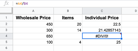
FIX: You need to populate the blank cell and enter in a value that is not zero.
Check for Invalid Data (Usually when using Average Formula)
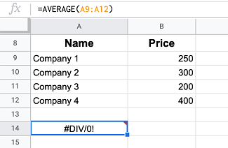
The AVERAGE formula is known to commonly cause the #DIV/0! error in Google Sheets because of invalid data.
In the example below we are trying to calculate the average of column A, however column A only contains names and names cannot have an average thus an error is thrown.
A sneaky way this error happens is when using the AVERAGEIF or AVERAGEIFS formula.
In the example below we are trying to calculate the average quote from each company, and we get an error for Mark’s Company.
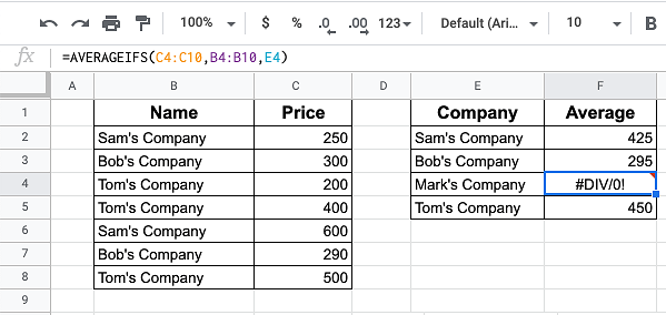
The reason this error is thrown is because we did not get a single quote from Mark’s Company and when trying to get the average the formula encounters a bunch of blank cells.
A mistake like this can be very common on big datasets. If we were getting quotes from hundreds of companies, then it is easy to wrongly assume we had a specific company in our dataset, when we actually did not.
Thus, it is very important to check if your formula is referring to any invalid data.
FIX: For this example, if we used Ctrl + F we would have quickly found out that we did not get a quote from Mark’s Company.
Check if Denominator Evaluates to Zero
A lot of times users think they are not dividing by zero when in fact their denominator somehow does evaluate to zero.
In the example below we are dividing 100 by the sum of the numbers in columns A1 to A6. The #DIV/0! error is thrown because the sum of A1:A6 is zero.
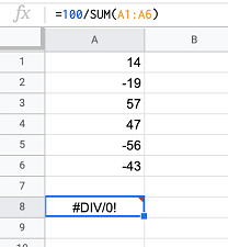
Here is a quick way to figure out if your denominator evaluates to zero:
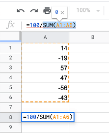
FIX: Highlight the denominator formula and you will see at the top what it equals to. (See image below)
Check if Formula Range Contains #DIV/0! Error
This is very common if you are working with a big dataset. As you saw in the blank cells example earlier column D4 contains the #DIV/0! error.
Now if we were to average all the values in column D, then we would also get the #DIV/0! error because our formula range (D2:D4) contains the error as well.
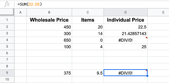
Even if we change the formula to the SUM of column D instead of average, we will still get the #DIV/0! error simply because the error exists in our formula range.
FIX: You need to look through your dataset and see if the error exists somewhere else. You can quickly do this by using Ctrl + F and searching for #DIV/0!
Use IFERROR
An option to hide the error is to surround your formula with IFERROR as seen in the example below.
=IFERROR(yourformula)
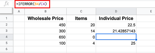
Simply replace yourformula with the original formula you had. So, if your formula was originally B4/C4, then you would enter in =IFERROR(B4/C4).
What surrounding your formula with IFERROR does is that if the formula throws an error then it will simply not display anything.
By using the formula below you can even customize what to write if the formula throws an error.
=IFERROR(yourformula, “Custom Message”)

Just replace yourformula with the original formula and Custom Message with whatever message you want displayed when an error occurs.