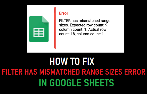
Some users have reported coming across an error while using the Filter feature in Google Sheets. The error which reads, Filter has mismatched range sizes, is usually due to your filtered values not having the same number of rows/columns.
However, there are also other reasons that can cause this error. In this article we will be exploring all the reasons this error occurs and will also be showing you how to fix this error.
Fix Filter Has Mismatched Range Sizes Error
The filter has mismatched range sizes error is usually caused by one of the following four reasons:
- Not starting at the same row
- Not ending at the same row
- Not including sheet name (if filtering data from a different sheet)
- Not starting/ending at the same column (for horizontally filtered data)
We will be showing you detailed examples of what each of these errors looks like and how to fix them to get the filter formula to work properly.
1. Not Starting at the Same Row
So, in this example we have a dataset that displays a bunch of basketball players and the number of points they have scored per game.
We want to filter this dataset to show only the basketball players that have scored more than 25 points per game.
So, we enter in the formula: =FILTER(A2:B10, B3:B10 > 25) and upon entering the formula we are given the “filter has mismatched range sizes” error.
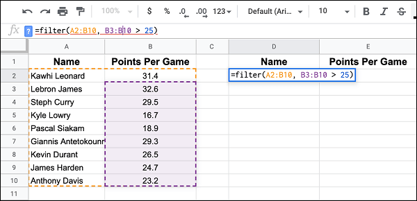
In this case the error is being caused because we are starting at different rows.
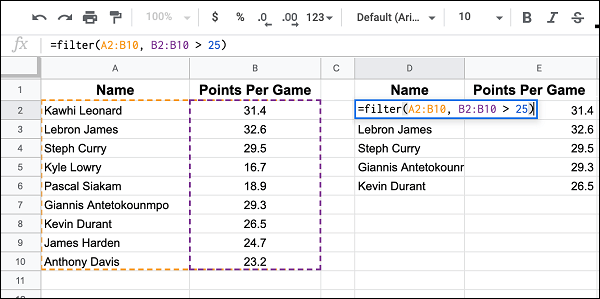
A2 is row 2, while B3 is row 3. If we change the formula to =FILTER(A2:B10, B2:B10 > 25), then the error will be fixed, and we will be shown all the players that have scored more than 25 points per game.
2. Not Ending at the Same Row
Similarly, the filter has mismatched range sizes error will also be displayed if you do not end at the same row.
In the example in the image below, the incorrect formula reads: =FILTER(A2:B10, B2:B9 > 25).
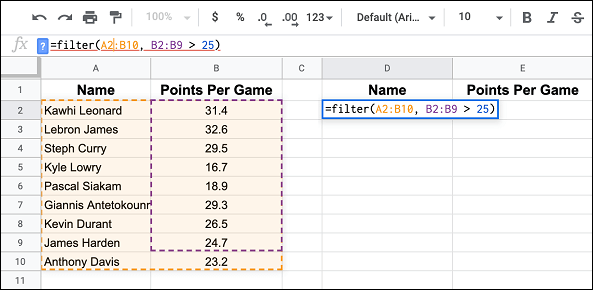
The first criteria is ending at row 10, while the second criteria is ending at row 9.
If we simply change the formula to =FILTER(A2:B10, B2:B10 > 25) then the formula will end up working correctly.

3. Not Including Sheet Name (For Data Filtered from Another Tab)
Another reason the filter has mismatched range sizes error can appear is if you are referring to data on another tab and you don’t include the sheet name in both criteria.
An example of this is in the image below, where the formula reads: =FILTER(Sheet1!A2:B10, B2:B10 > 25).
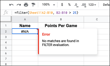
When referring to data from another sheet, it is important that you include the sheet name in both criteria.
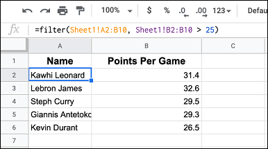
If the formula is changed to: =FILTER(Sheet1!A2:B10, Sheet1!B2:B10 > 25), then the error is fixed and the dataset is filtered.
4. Not Starting/Ending at the Same Column (For Horizontally Filtered Data)
If you are filtering a horizontal dataset, then to fix the filter has mismatched range sizes error, you need to make sure that you are starting and ending at the same column.
In the example in the image below, the formula is =FILTER(B1:2, C2:2 > 25).
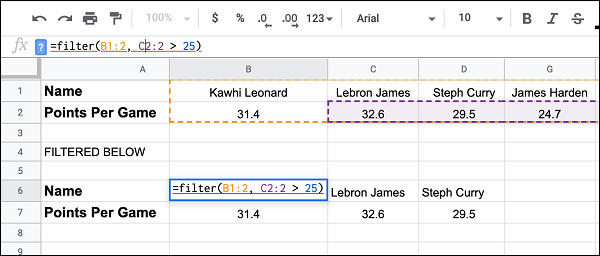
Both criteria are not starting at the same value, one starts at column B, while the other starts at column C.
Changing the formula to =FILTER(B1:2, B2:2 > 25) will fix the error.
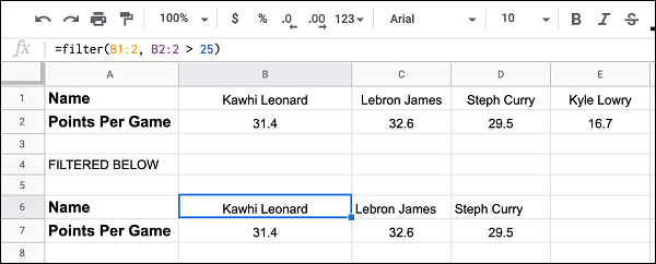
Another time the error can happen is if you do not end at the same column. In the example below the formula reads: =FILTER(B1:2, B2:G2 > 25)
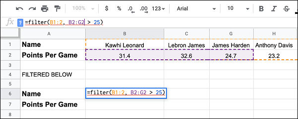
In this case the criteria are not ending at the same column number.
Changing the formula to =FILTER(B1:2, B2:2 > 25) solves the problem and leads to the data being filtered.