A lot of people choose to color alternate rows of a spreadsheet to make it more readable.
Previously color alternating rows in Google Sheets was a lengthy process, however Google has introduced a new built-in feature that makes the task relatively easy.
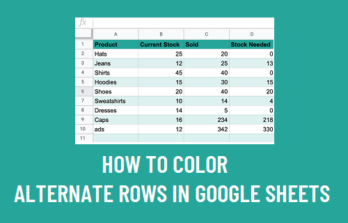
Color Alternate Rows in Google Sheets
We will be changing a plain dataset into one with alternatively colored rows.
1. Select the entire dataset or the rows you want to color alternate
2. Click on Format from the top menu and then click on Alternating Colors

3. To choose from the default styles, choose a style under the heading Default styles
4. To choose a custom style, under the header custom style, choose colors for the header, color 1, and color 2.
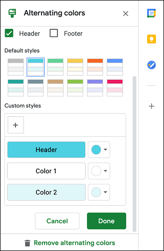
5. Click on Done to save the changes
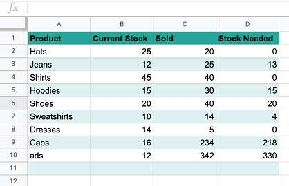
As you can see our plain dataset, now has alternating colored rows.
What Happens if you Make Changes to the Dataset?
If you add more rows to the dataset then Google Sheets will automatically color alternate those rows as well. Even if rows are added in between the dataset Google Sheets will automatically adjust the color alternation of the entire table.
On the other hand, if you delete rows from the bottom of a dataset then sometimes the color of the deleted row stays, and you will need to remove it manually.
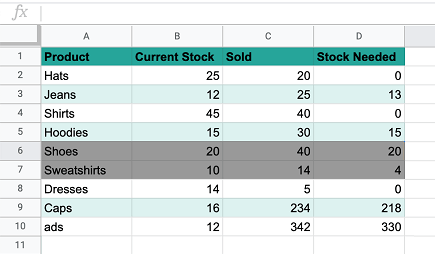
If you decide to manually color any rows in the dataset with a different color, then the new color overrides the alternating colors and the rest of the table ignores this row and continues the regular color alternating pattern, as seen below.
Remove Color Alternating Rows in Google Sheets
At any time, you can easily remove color alternating rows in Google Sheets.
1. Click on any cell in the colored dataset.
2. Click on Format > Alternating Colors

3. Click on Remove Alternating Colors option
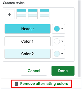
The dataset will now return back to how it was before the alternate rows were colored.