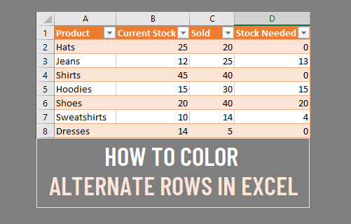
To make your data easier to read, you may want to color alternate rows in Excel. Excel provides built in functionality to do this and even alternatively colors newly added rows.
Color Alternate Rows in Excel
To use the built in Excel feature, you first need to format your data as a table.
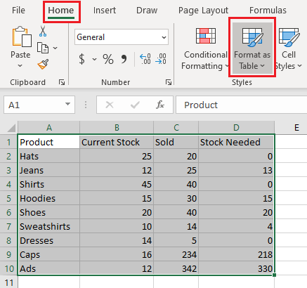
1. Select the entire dataset or only the rows you want to color alternate
2. Click on Home from the top menu and then click on Format as Table (See image below)
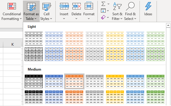
3. From the dropdown menu, choose a style that has alternating colored rows.
4. If your table has a header make sure the ‘My table has headers’ option is selected and then click on Ok

The table will now have alternatively colored rows, making it much easier to read.
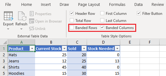
Tip: To shade columns instead of rows, simply select a cell in the table, click on Design and check the Banded Columns option and uncheck the Banded Rows option.
Convert to Range
If you do not want to keep your dataset as a table, but still want to keep the alternately colored rows, then you can convert the dataset back to a range.
1. Select any cell in the table, and then click on Table Design (‘Table’ on Mac) from the top menu
2. Next click on Convert to Range
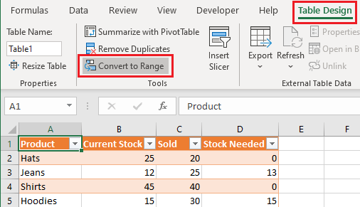
3. From the pop-up, click on Yes
The table will now be converted to a range, as you can see below.
Change or Remove Alternating Row Colors
If you get bored of the color you chose or for any reason want to change/remove the color, here is how you can do it:
1. Select any cell in the table, and then click on Table Design (‘Table’ on Mac) from the top menu
2. Click on the dropdown that contains previews of table styles and then select a new color if you want to change the color

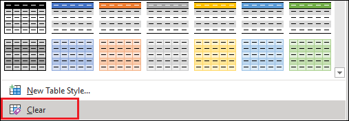
3. To remove the color and go back to a plain table, click on Clear from the bottom
