Some people prefer having a dataset with blank spaces, but others absolutely detest it.
Instead of manually finding and deleting each blank row, you can have Excel do the hard work for you.
In this tutorial we will be showing you 2 different ways to delete blank rows in Excel.
Easy Way to Remove Blank Rows in Excel
Excel’s find and select function makes it very easy to remove blank rows.
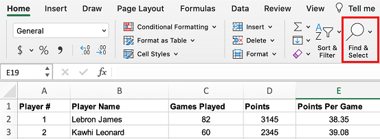
1. Make sure you are on the Home tab and click on Find & Select.
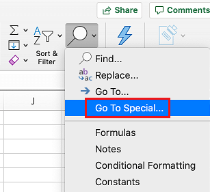
2. From the dropdown menu, click on Go to Special
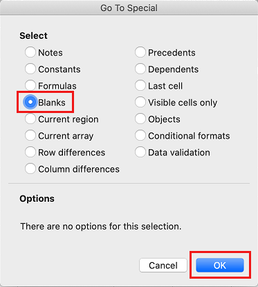
3. Select Blanks from the pop-up window and then click on Ok
You will now notice that all the blank cells have been selected.

Tip: In case Excel has selected a blank cell that you do not want to delete (like in the example below) then simply hold the Ctrl key and click on the cell to unselect it. On Mac computers, press the Command key and then click on the cell to unselect it.

4. Click on the Delete option (See image below)
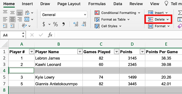
The blank rows will now be deleted from your dataset.
Traditional Way to Remove Blank Rows
Before Excel introduced the Find & select shortcut, most users would delete blank rows using the filter and delete method.
Here is how this method works.
1. Select your entire dataset (See image below)

2. Click on the Data Tab and then click on the Filter option
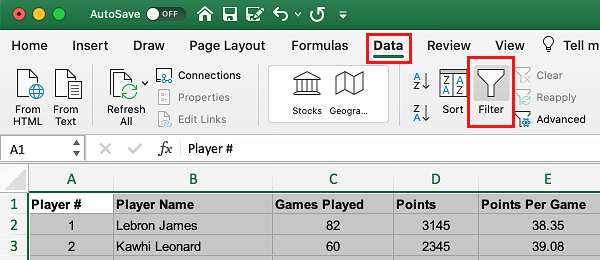
3. Click on the dropdown icon from any of the columns
![]()
4. Now click on the Select All option to uncheck all the boxes.

5. Next click on the (Blanks) option to only display the blank cells.

6. Select all the blank rows in your dataset (the row number will be highlighted in blue)

Tip: To select rows, click on the first blue row and then while holding down the Shift key, click on the last blue row.
7. Now right click on any of the blue numbers and then click on Delete Row from the dropdown menu.
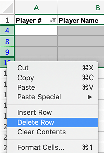
8. Now click on the Filter icon from the top once again and you will now see your dataset displayed with all the blank rows removed.
